2 Manipulate
Learning Objectives
Read online table.
Download a tabular file, in commonly used comma-separated value (*.csv) format, from the URL of a dataset on an ERDDAP server.
Read a CSV file into a
data.frame()using base Rutils::read.csv().
Show the table.
Show the
data.framein the R console.Render the table into HTML with
DT::datatable().
Wrangle with
tibble,dplyr,tidyrandpurrr.Convert the
data.frameto a tidyversetibble()and show it again, now with a more informative summary.Pipe commands with
%>%fromdplyrfor feeding the output of the function on the left as the first input argument to the function on the right.Select columns of information with
select(), optionally using select operators likestarts_with().Filter rows of information based on values in columns with
filter().Mutate a new column with
mutate(), possibly derived from other column(s).Summarize all rows with
summarize(). Precede this withgroup_by()to summarize based on rows with common values of a given column.Nest tables inside of tables with a
tibbleand tidyr’snest(). Build a linear model object (lm()) into another list column per grouping using purrr’smap(). Extract values from this model object as double withmap_dbl().
Tips for using RStudio
Always launch RStudio from an
*.Rprojfile so it sets the working directory.Use the Visual Markdown Editor (version 1.4+; see menu RStudio > About RStudio to check your version) to easily create Markdown in your Rmarkdown document.
2.1 Read online table
In this first set of exercises we’ll read marine ecological indicators from California Current - Home | Integrated Ecosystem Assessment (IEA). These datasets are also being served by an ERDDAP server (which is “a data server that gives you a simple, consistent way to download subsets of scientific datasets in common file formats and make graphs and maps.”).
2.1.1 Create manipulate.Rmd in r3-exercises
Open your Rstudio project for the r3-exercises by double-clicking on the r3-exercises.Rproj file (from Windows Explorer in Windows; Finder in Mac). This will set the working directory in the R Console to the same folder.
In RStudio menu, File -> New File -> R Markdown… I suggest giving it a title of “Manipulate” and saving it as manipulate.Rmd. Let’s delete everything after the first R chunk, which is surrounded by fenced backticks:
```{r setup, include=FALSE}
knitr::opts_chunk$set(echo = TRUE)
```
And create a new heading and subheading:
## Read online table

### Download table (`*.csv`)
2.1.2 Get URL to CSV
Please visit the ERDDAP server https://oceanview.pfeg.noaa.gov/erddap and please do a Full Text Search for Datasets using “cciea” in the text box before clicking Search. These are all the California Current IEA datasets.
From the listing of datasets, please click on data for the “CCIEA Anthropogenic Drivers” dataset.
Note the filtering options for time and other variables like consumption_fish (Millions of metric tons) and cps_landings_coastwide (1000s metric tons). Set the time filter from being only the most recent time to the entire range of available time from 1945-01-01 to 2020-01-01.
Scroll to the bottom and Submit with the default .htmlTable view. You get an web table of the data. Notice the many missing values in earlier years.
Go back in your browser to change the the File type to .csv. Now instead of clicking Submit, click on Just generate the URL. Although the generated URL lists all variables to include, the default is to do that, so we can strip off everything after the .csv, starting with the query parameters ? .
2.1.3 Download CSV
Let’s use this URL to download a new file in a new R Chunk (RStudio menu Code -> Insert Chunk). Paste the following inside your R Chunk:
# set variables
csv_url  <- "https://oceanview.pfeg.noaa.gov/erddap/tabledap/cciea_AC.csv"
# if ERDDAP server down (Error in download.file) with URL above, use this:
#    csv_url <- "https://raw.githubusercontent.com/noaa-iea/r3-train/master/data/cciea_AC.csv"
dir_data <- "data"

# derived variables
csv <- file.path(dir_data, basename(csv_url))

# create directory
dir.create(dir_data, showWarnings = F)

# download file
if (!file.exists(csv))
  download.file(csv_url, csv)
Then click the green Play button to execute the commands in the R Console. After the last command you should see something like:
trying URL 'https://oceanview.pfeg.noaa.gov/erddap/tabledap/cciea_AC.csv'
downloaded 53 KB
2.1.4 Read table read.csv()
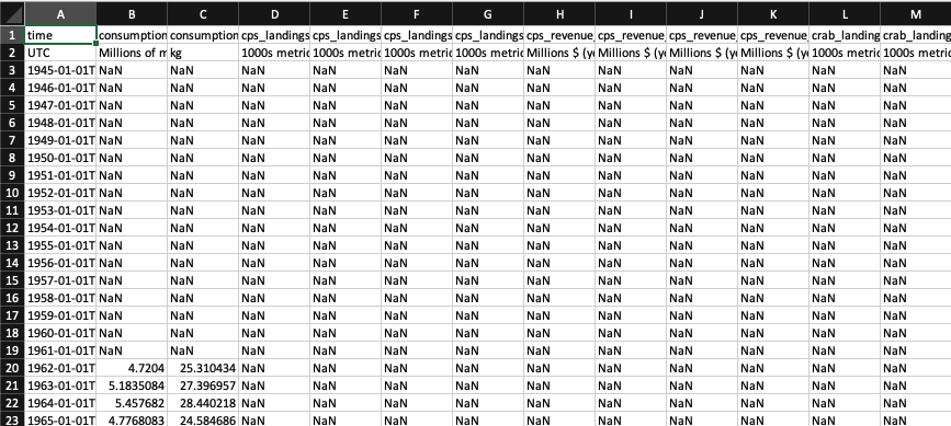
Now open the file by going into the Files RStudio pane, More -> Show Folder in New Window. Then double click on data/cciea_AC.csv to open in your Spreadsheet program (like Microsoft Excel or Apple Pages or LibreOffice Calc). Mine looks like this:
Let’s try to read in the csv by adding a new subsection in your Rmarkdown file:
### Read table `read.csv()`Then create a new R Chunk and add the following lines to the R chunk:
# attempt to read csv
d <- read.csv(csv)

# show the data frame
d
Note how the presence of the 2nd line with units makes the values character <chr> data type:
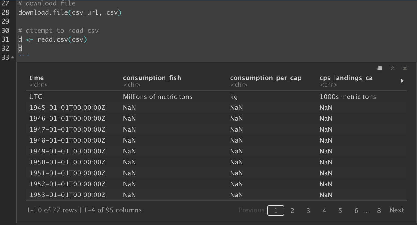
But we want numeric values. So we could manually delete that second line of units or look at the help documentation for this function (?read.csv in Console pane; or F1 key with cursor on the function in the code editor pane). Notice the skip argument, which we can implement like so:
# read csv by skipping first two lines, so no header
d <- read.csv(csv, skip = 2, header = FALSE)
d

# update data frame to original column names
names(d) <- names(read.csv(csv))
d

# update for future reuse (NEW!)
write.csv(d, csv, row.names = F)
You can run above one line at a time with Code -> Run Selected Lines (note the keyboard shortcut, which depends on your operating system). This will allow you to see how the data.frame d evolves. When running the w
2.1.5 Show table DT::datatable()
Next, let’s render your Rmarkdown to html by clicking on Knit button (with the blue ball of yarn). Notice how all those times of outputting d show the full dataset with each line prefixed by a comment. There are many prettier ways to show tables in Rmarkdown. We’ll use the DT R package to start.
You’ll need to install the R package if you don’t already have it. Check by searching for it in the Packages pane and Install if missing.
Let’s start by commenting the previous instances of d (lines 36, 40, 44 for me) by prefixing with a #. Then try adding this subsection:
### Show table `DT::datatable()`And in a new R chunk:
# show table
DT::datatable(d)
Then Knit again to see the updated table display, which defaults to paging through results, showing alternating gray backgrounds and providing search and sort abilities. Check out the function help (?DT::datatable in R Console; or F1 with cursor over function in editor) and R package website DT for more.
Also note how we can call a function explicitly with the R package like DT::datatable(d) or load the library and use the function without the explicit R package referencing:
library(DT)
datatable(d)
2.2 Wrangle data
Now that we’ve learned how to read a basic data table, let’s “wrangle” with dplyr, tidyr and purrr:
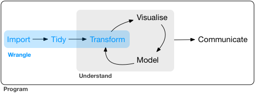
Data “wrangling” loosely encompasses the Import, Tidy and Transform steps. Source: 9 Introduction | R for Data Science
Let’s create a new section and subsection in your Rmd:
## Wrangle data

### Manipulate with `dplyr`
2.2.1 Install R packages
Be sure you have the R packages dplyr, tidyr and purrr installed via the Packages pane. Search (magnifying glass) for them and if missing, use the Install button.
2.2.2 Manipulate with dplyr
There’s a few things we’ll want to do next to make this data.frame more usable:
Convert the
data.frameto atibble, which provides a more useful summary in the default output of the R Console to include only the first 10 rows of data and the data types for each column.Transform the
timecolumn to an actualas.Date()column using dplyr’smutate().Column select with dplyr’s
select()to those starting with “total_fisheries_revenue” usingstarts_with().Row select with dplyr’s
filter()to those starting within the last 40 years, i.e.time >= as.Date("1981-01-01").
Create a new R Chunk (RStudio menu Code -> Insert Chunk) and insert within the fenced code block the following:
library(DT)
library(dplyr)

d <- d %>%
  # tibble
  tibble() %>%
  # mutate time
  mutate(
    time = as.Date(substr(time, 1, 10))) %>%
  # select columns
  select(
    time,
    starts_with("total_fisheries_revenue")) %>%
  # filter rows
  filter(
    time >= as.Date("1981-01-01"))

datatable(d)
Next, Run the the chunk with the green Play button. Knit your document to see the update output table.
2.2.3 Tidy with tidyr
Now, we’re ready to “tidy” up our data per the definition in the Data Import Cheatsheet:
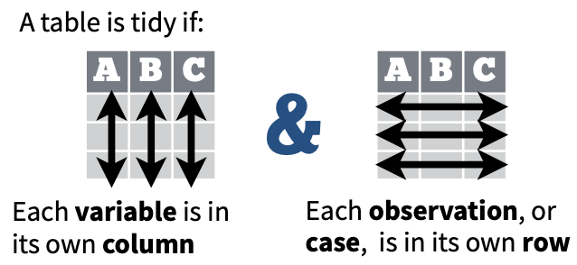
We’ll see how this transformation of the data structure from wide to long is especially useful in the next section when we want to summarize fisheries revenue by region.
Add a new subsection in your Rmd:
### Tidy with `tidyr`And a new R Chunk:
library(tidyr)

d <- d %>%
  pivot_longer(-time)

datatable(d)
2.2.4 Summarize with dplyr
Now that we have the data in long format, we can:
Mutate a new
regionfrom the original full columnnameby using stringr’sstr_replace()function.Select for just the columns of interest (we no longer need
name).Summarize by
region, which we want to firstgroup_by(), thensummarize()themean()ofvalueto a new columnavg_revenue).Format the
avg_revenueas a currency with DT’sformatCurrency()).
Add a new subsection in your Rmd:
### Summarize with `dplyr`And a new R Chunk:
library(stringr)

d <- d %>%
  mutate(
    region = str_replace(name, "total_fisheries_revenue_", "")) %>%
  select(time, region, value)
datatable(d)
d_sum <- d %>%
group_by(region) %>%
summarize(
avg_revenue = mean(value))
datatable(d_sum) %>%
formatCurrency("avg_revenue")2.2.5 Apply functions with purrr on a nest’ed tibble
One of the major innovations of a tibble is the ability to store nearly any object in the cell of a table as a list column. This could be an entire table, a fitted model, plot, etc. Let’s try out these features driven by the question: What’s the trend over time for fishing revenue by region?
The creation of tables within cells is most commonly done with tidyr’s
nest()function based on a grouping of values in a column, i.e. dplyr’sgroup_by().The
purrrR package provides functions to operate on list objects, in this case the nested data. and application of functions on these data with purrr’smapfunction. We can feed thedataobject into an anonymous function where we fit the linear modellm()and return a list object. To then extract the coefficient from the modelcoef(summary()), we want to return a type of double (not another list object), so we use themap_dbl()function.
Add a new subsection in your Rmd:
### Apply functions with `purrr` on a `nest`'ed `tibble`And a new R Chunk:
library(purrr)

n <- d %>%
  group_by(region) %>%
  nest(
    data = c(time, value))
n
## # A tibble: 4 × 2
## # Groups: region [4]
## region data
## <chr> <list>
## 1 ca <tibble [40 × 2]>
## 2 coastwide <tibble [40 × 2]>
## 3 or <tibble [40 × 2]>
## 4 wa <tibble [40 × 2]>n <- n %>%
mutate(
lm = map(data, function(d){
lm(value ~ time, d) } ),
trend = map_dbl(lm, function(m){
coef(summary(m))["time","Estimate"] }))
n## # A tibble: 4 × 4
## # Groups: region [4]
## region data lm trend
## <chr> <list> <list> <dbl>
## 1 ca <tibble [40 × 2]> <lm> -0.0117
## 2 coastwide <tibble [40 × 2]> <lm> -0.00454
## 3 or <tibble [40 × 2]> <lm> 0.00379
## 4 wa <tibble [40 × 2]> <lm> 0.00333n %>%
select(region, trend) %>%
datatable()2.3 Rmarkdown output options
If you’d like to render your Rmarkdown into HTML with a table of contents (toc), showing up to 3rd level headings (i.e. ### Heading; use toc_depth: 3) and have a floating menu (toc_float), along with the ability to Show (or Hide) your Code Chunks (code_folding), then replace this default front matter yaml:
output: html_documentwith:
output:
  html_document:
    toc: true
    toc_depth: 3
    toc_float: true
    code_folding: "show"
For details, see 3.1 HTML document | R Markdown: The Definitive Guide.
Further Reading
Cheatsheets
RStudio Cheatsheets (most also available via RStudio menu Help > Cheat Sheets):
- RStudio IDE: RStudio interface
- Data Import:
readr,tidyr - Data Transformation:
dplyr - Apply functions with
purrr - Dates and Times Cheatsheet:
lubridate - Work with Strings Cheatsheet:
stringr - Regular Expressions Cheatsheet:
stringr+ regex - Tidy Evaluation with rlang: advanced topics on how to use non-standard evaluation (i.e. unquoted strings referencing columns or other variables), especially for creating functions to handle tidy data
Further Learning Objectives
For another day…
Pipe commands with
%>%fromdplyrfor feeding the output of the function on the left as the first input argument to the function on the right.
Read online table.
Download a tabular file, in commonly used comma-separated value (*.csv) format, from the URL of a dataset on an ERDDAP server.
Read a CSV file into a
data.frame()using base Rutils::read.csv()and compare with the tidyverse R functionreadr::read_csv(). Understand the difference in how characters are handled as factors versus character.APIs, or application programming languages, provide a consistent way to query an online resource (with query parameters in a GET URL or longer forms with a POST from a form) and return information (typically as JSON), on reading csv directly from URL and using
rerddapR package to access ERDDAP, which is an API that you could directly read withhttrR package. For building your own API, seeplumber(and REST APIs with Plumber Cheatsheet).
Show the table.
Show the
data.framein the R console. Display asummary(). Convert thedata.frameto a tidyversetibble()and show it again, now with a more informative summary.View()the table in RStudio.Render the table into HTML with
DT::datatable(). Render the Rmarkdown document topdfanddocxto see the shortcomings of this htmlwidget in these formats. Useknitr::kable()for simple tables and thehuxtableR package for these non-HTML formats.
Manipulate with
dplyr.See Data Transformation Cheatsheet.
Select columns of information with
select(), optionally using select operators likestarts_with(),ends_with()andeverything(). Userename()to only rename existing columns.Filter rows of information based on values in columns with
filter(). Slice data based on row numbers.Arrange rows by values in one or more columns with
arrange(). Arrange in ascending (default) or descending (desc()) order. Use factors to customize the sort order.Pull values with
pull()into a singlevector(versus the defaultdata.frameoutput).Mutate a new column with
mutate(), possibly derived from other column(s). Useglue::glue()to combine character columns,stringrR package to manipulate character strings, andlubridateR package for dates.
See Dates and Times Cheatsheet, Work with Strings Cheatsheet, Regular Expressions Cheatsheet.Summarize all rows with
summarize(). Precede this withgroup_by()to summarize based on rows with common values of a given column.Join two tables on a common column with
left_join()(all from left; matching from right) orinner_join()(matching from left and right). Get unmatched values withanti_join().
Nest tables Unnest. Get climatology by group as data, save linear model in cell, plot in cell. List column concept. Purrr
purrr::map()function.Create a function to use an argument.
See Tidy Evaluation with rlang CheatsheetPivot tables between wide and long formats. How would you summarize by group without a long format? A: it would be a painful for loop.
Relational database concepts with sqlite. And using
tbl(con, "table"),sql_show()andcollect(). Migrate from CSV to sqlite to PostgreSQL to PostGIS to BigQuery. Dplyr as the middle layer (and dbplyr). See db.rstudio.com for more, especially on previewing SQL results withconn. Compare dplyr commands to SQL.See Databases using R.
Compare all of the above tidyverse operations with base R functions and note the readability (i.e. cognitive load) for understanding the analyses.