3 Map

Learning Objectives

3.1 Read Spatial Data

Open your r3-exercises.Rproj to launch RStudio into that project and set the working directory.

Create a new Rmarkdown file (RStudio menu File > New file > Rmarkdown…) called map.Rmd. Insert headers like last time followed by Chunks of R code according to the examples provided below.

I’ll be copy/pasting during the demonstration but I encourage you to type out the text to enhance understanding.

3.1.1 Install packages

# require() is like library() except returns FALSE if missing (vs error)
if (!require(librarian)){
  install.packages("librarian")
  library(librarian)
}
# librarian::shelf() is like library() except installs package if missing, 
#   even from Github if include owner/repo
shelf(
  NOAA-EDAB/ecodata,
  sf)
# librarian before version 1.8.1, got error:
#   download from 'https://api.github.com/repos/NOAA-EDAB/ecodata/tarball/HEAD' failed

3.2 Get spatial data

ecodata::epu_sf

## Simple feature collection with 4 features and 3 fields
## Geometry type: MULTIPOLYGON
## Dimension:     XY
## Bounding box:  xmin: -77 ymin: 35.8327 xmax: -65.66667 ymax: 44.66667
## Geodetic CRS:  NAD83
##   EPU Shape_Leng Shape_Area                       geometry
## 0  GB   16.33086   6.162033 MULTIPOLYGON (((-66.5 42.16...
## 1 GOM   32.20684   7.545063 MULTIPOLYGON (((-69.26278 4...
## 2  SS   20.52712   3.350430 MULTIPOLYGON (((-67.54 44.6...
## 3 MAB   83.38407  15.695390 MULTIPOLYGON (((-75.97418 3...

epu_sf <- ecodata::epu_sf %>% 
  st_transform(4326)

So we see a geometry list column.

class(epu_sf)

## [1] "sf"         "data.frame"

# "sf"         "data.frame"
g1 <- epu_sf$geometry[1]
# see in Environment pane, expand g1

plot(epu_sf)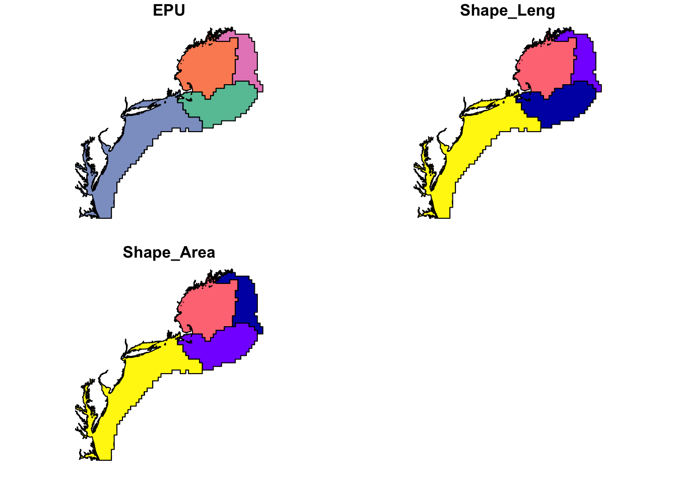

plot(epu_sf["EPU"])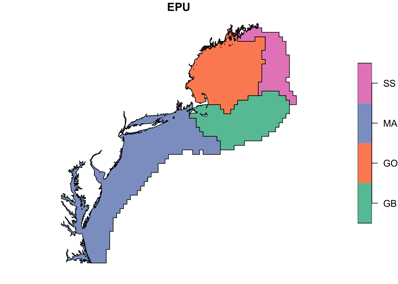

Where in the world is this?

shelf(mapview)

mapview(epu_sf)

shelf(leaflet)

leaflet() %>% 
  #addTiles() %>%
  addProviderTiles(providers$Esri.OceanBasemap) %>% 
  addPolygons(data = epu_sf)

3.3 Group by

sf is “tidy”

3.4 Extract from erddap

shelf(
  here,
  rerddap)

sst_gd_rds <- here("data/sst_gd.rds")

epu_bb <- st_bbox(epu_sf)
epu_bb

##      xmin      ymin      xmax      ymax 
## -77.00000  35.83270 -65.66667  44.66667

sst_info <- info('jplMURSST41mday')
sst_info

## <ERDDAP info> jplMURSST41mday 
##  Base URL: https://upwell.pfeg.noaa.gov/erddap/ 
##  Dataset Type: griddap 
##  Dimensions (range):  
##      time: (2002-06-16T00:00:00Z, 2021-06-16T00:00:00Z) 
##      latitude: (-89.99, 89.99) 
##      longitude: (-179.99, 180.0) 
##  Variables:  
##      mask: 
##      nobs: 
##      sst: 
##          Units: degree_C

if (!file.exists(sst_gd_rds)){
  sst_gd <- griddap(
    sst_info,
    fields    = "sst",
    time      = c("2020-06-16", "2021-06-16"),
    longitude = epu_bb[c("xmin", "xmax")],
    latitude  = epu_bb[c("ymin", "ymax")])
  saveRDS(sst_gd, file = sst_gd_rds)  
}
sst_gd <- readRDS(sst_gd_rds)

sst_gd

## <ERDDAP griddap> jplMURSST41mday
##    Path: [~/Library/Caches/R/rerddap/6d0dbbf4f950f8dc4ffca5dd9b2cf661.nc]
##    Last updated: [2021-07-12 17:47:17]
##    File size:    [52.2 mb]
##    Dimensions (dims/vars):   [3 X 1]
##    Dim names: time, latitude, longitude
##    Variable names: Sea Surface Temperature Monthly Mean
##    data.frame (rows/columns):   [13046670 X 4]
## # A tibble: 13,046,670 × 4
##    time                   lat   lon   sst
##    <chr>                <dbl> <dbl> <dbl>
##  1 2020-06-16T00:00:00Z  35.8 -77      NA
##  2 2020-06-16T00:00:00Z  35.8 -77.0    NA
##  3 2020-06-16T00:00:00Z  35.8 -77.0    NA
##  4 2020-06-16T00:00:00Z  35.8 -77.0    NA
##  5 2020-06-16T00:00:00Z  35.8 -77.0    NA
##  6 2020-06-16T00:00:00Z  35.8 -76.9    NA
##  7 2020-06-16T00:00:00Z  35.8 -76.9    NA
##  8 2020-06-16T00:00:00Z  35.8 -76.9    NA
##  9 2020-06-16T00:00:00Z  35.8 -76.9    NA
## 10 2020-06-16T00:00:00Z  35.8 -76.9    NA
## # … with 13,046,660 more rows

names(sst_gd)

## [1] "summary" "data"

shelf(
  dplyr,
  ggplot2,
  mapdata)

# coastline
coast <- map_data(
  "worldHires", 
  xlim = epu_bb[c("xmin", "xmax")],
  ylim = epu_bb[c("ymin", "ymax")],
  lforce = "e")

sst_df_last <- sst_gd$data %>%
    filter(time == max(time))

# summary(sst_last)

ggplot(
  data = sst_df_last, 
  aes(x = lon, y = lat, fill = sst)) +
  geom_polygon(
    data = coast,
    aes(x = long, y = lat, group = group), fill = "grey80") +
  geom_tile() +
  scale_fill_gradientn(
    colors = rerddap::colors$temperature, na.value = NA) +
  theme_bw() + 
  ylab("Latitude") + 
  xlab("Longitude") +
  ggtitle("Latest SST")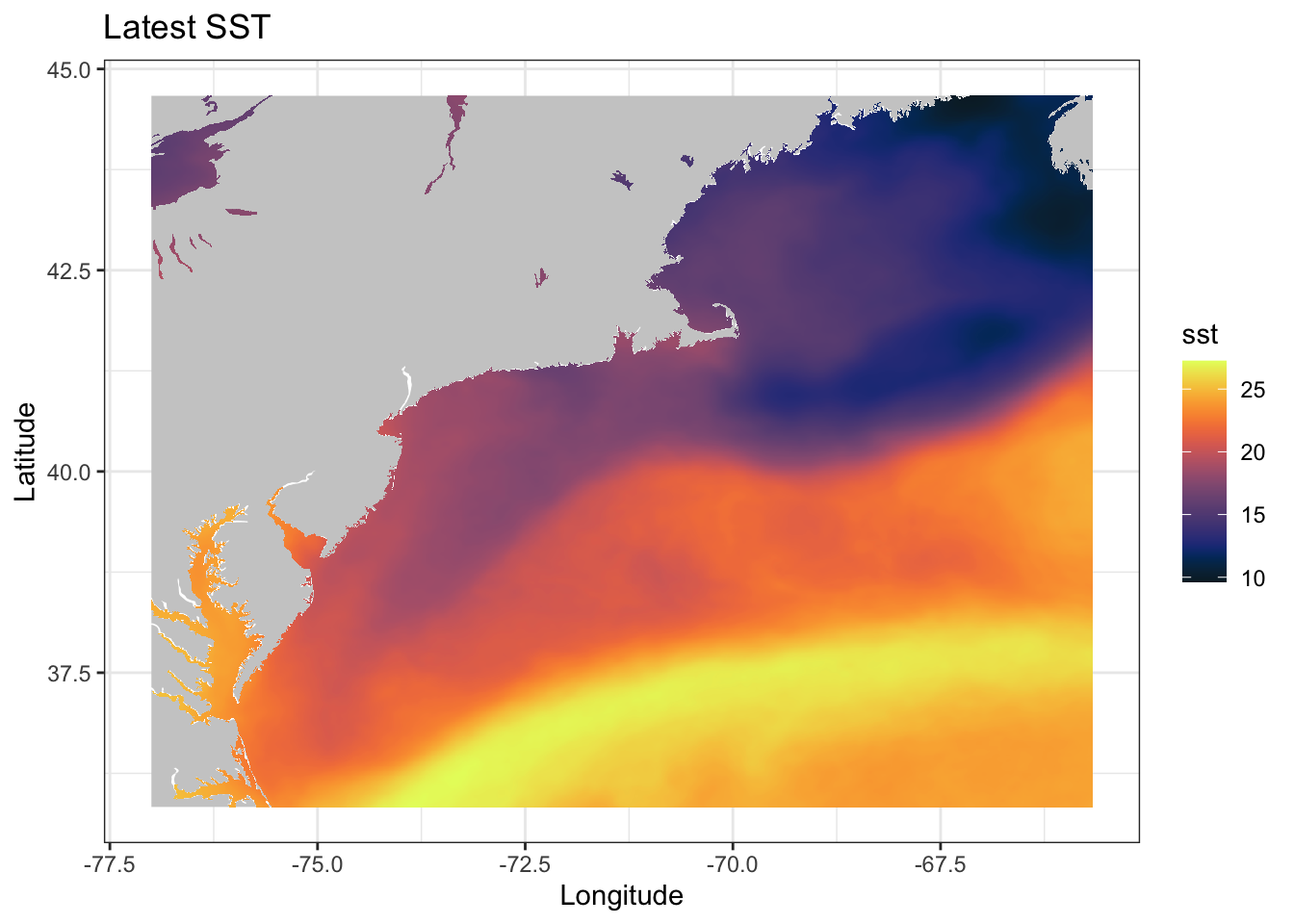

shelf(
  purrr,
  raster,
  sp,
  tidyr)
select <- dplyr::select

sst_tbl <- tibble(sst_gd$data) %>%
  mutate(
    # round b/c of uneven intervals
    #   unique(sst_gd$data$lon) %>% sort() %>% diff() %>% table()
    #     0.0099945068359375 0.0100021362304688
    lon  = round(lon, 2),
    lat  = round(lat, 2),
    date = as.Date(time, "%Y-%m-%dT00:00:00Z")) %>%
  select(-time) %>% 
  filter(!is.na(sst)) # 13M to 8.8M rows

sst_tbl_mo <- sst_tbl %>% 
  nest(data = c(lat, lon, sst)) %>% 
  mutate(
    raster = purrr::map(data, function(x) {
      #browser()
      sp::coordinates(x) <- ~ lon + lat
      sp::gridded(x)     <- T
      raster::raster(x)
    }))

sst_stk <- raster::stack(sst_tbl_mo$raster)
names(sst_stk) <- strftime(sst_tbl_mo$date, "sst_%Y.%m")
raster::crs(sst_stk) <- 4326

shelf(stringr)

epu_sst_avg <- raster::extract(sst_stk, epu_sf, fun = mean, na.rm = T)
epu_sst_sd  <- raster::extract(sst_stk, epu_sf, fun = sd, na.rm = T)

epu_sst_tbl <- rbind(
  epu_sst_avg %>% 
    as_tibble() %>% 
    cbind(
      EPU  = epu_sf$EPU,
      stat = "mean") %>% 
    pivot_longer(-c(EPU, stat)),
  epu_sst_sd %>% 
    as_tibble() %>% 
    cbind(
      EPU = epu_sf$EPU,
      stat = "sd") %>% 
    pivot_longer(-c(EPU, stat))) %>% 
  mutate(
    EPU  = as.character(EPU),
    date = as.double(str_replace(name, "sst_", ""))) %>% 
  select(-name) %>% 
  pivot_wider(
    names_from  = EPU, 
    values_from = value)

shelf(dygraphs)

epu_sst_tbl %>% 
  filter(stat == "mean") %>% 
  select(-stat) %>% 
  dygraph()